
1. Description of the problem
Simulation results of the problem of aircraft landing are given below. The penultimate stage of the landing process is considered. At this stage, the aircraft should descent along a rectilinear glide path (Fig.1). The stage terminates when the aircraft passes the runway threshold. The objective of the useful control is to guide the deviations of the parameters of the aircraft motion to some given tolerances at the terminal instant. Together with the useful control, the aircraft is affected by a wind disturbance. A peculiarity of the problem formulation is that the useful control is geometrically constrained, whereas there is no any a priori constraint for the wind.
|
|
| Fig.1. Descending glide path |
When modeling, the following situation is considered. The aircraft motion starts in 8 kilometers before the runway threshold. The nominal motion is the rectilinear descending from 390 m down to 15 m during approximately 120 sec. The nominal wind is taken as a cross-wind with the velocity 5 m/sec. The simulated motion starts with +40 m of vertical deviation (that is, from the height of 430 m) and with 80 m of lateral deviation.
2. The aircraft dynamics
The aircraft dynamics is described by a non-linear differential system of the 16th order [1]. The phase variables are: three geometric coordinates of the mass center, three angular variables (the angles of pitch, roll, and yaw), and 6 corresponding linear and angular velocities. Four additional variables describes the inertiality of the servomechanisms. The system is affected by two players. The first of them is the useful control consisting of four scalar components: the command levels of the thrust, command deviations of the elevators and rudder, and deviations of the ailerons. The last four differential equations in the system smooth the command values and transform them to the actual states of the control devices. The second player is the wind disturbance, which is presented by a three-dimensional wind velocity vector.
3. The first player's control
As the first player's control, a robust control [2] was applied. The main features of the control are the following: at first, it should lead the system to the terminal set if the disturbance is lower then some critical level; at second, the weaker the disturbance is, the weaker should be the parrying control.
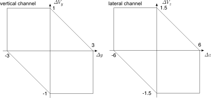
Since the suggested method for constructing robust control is oriented to linear systems, the original nonlinear system is linearized along the nominal trajectory. After linearization, it disjoins into two independent (or almost independent) linear subsystems: of the vertical and lateral motions. On the basis of each of these subsystems, an auxiliary differential game is formulated for each channel. The terminal sets, to which the system should be guided at the terminal instant, are shown in Fig.2. For the vertical channel, the set is given in the space vertical deviation × vertical velocity. Similarly, for the lateral channel, the set is in the space lateral deviation × lateral velocity. Value of all other components of the phase vector at the terminal instant are ignored.
|
| Fig.2. The terminal sets |
The linear subsystems are used to construct the first player's control. During simulation, the original non-linear system has been used.
For simulation, the following values have been taken as critical for the wind velocities: the longitudinal wind ≤ 6 m/sec, the vertical wind ≤ 4 m/sec, the lateral wind ≤ 10 m/sec.
4. The second player's control
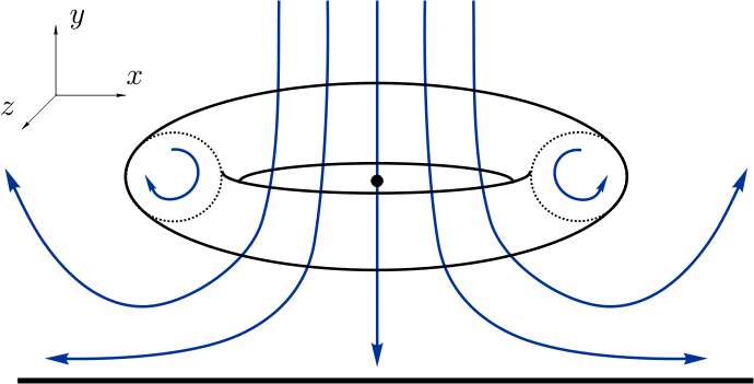
As the second player's control, a wind microburst model suggested by M.Ivan in [3] was applied. A wind microburst is a natural phenomenon appearing when a descending air current strikes the ground and flows off horizontally. Schematically, the model is shown in Fig.3. The torus is a zone of relatively still mass of air; there is turbulence around it.
|
| Fig.3. The microburst model |
When passing the microburst zone, at first, the aircraft meets a cross-wind, which changes quite fast to descending one and, finally, a tail-on wind. The wind velocity almost does not affect the velocity of the aircraft with respect to the ground. But the air speed depends significantly on the wind velocity, so the lifting power does. The cross-wind increases the airspeed and the lifting power. Thus, the aircraft starts to ascend above the glide path, and to return back the pilot should decrease the thrust. Subsequent change of the wind to tail-on, on the contrary, leads to decreasing of the air speed and the lifting power. Due to this, the aircraft dips that often leads to a crash. The correct action in this case is to increase the thrust quickly.
For simulation, the following parameters of the microburst have been taken. The center of the microburst (of the torus in Fig.3) is located in 4000 m before the runway threshold, in 500 m aside and in 600 m above the ground. The radius of the central ring of the torus equals 1200 m, radius of the torus section is 480 m. The wind velocity in the central point was taken equal to 10 m/sec; the maximal value of the wind velocity was 18 m/sec.
5. Simulation results
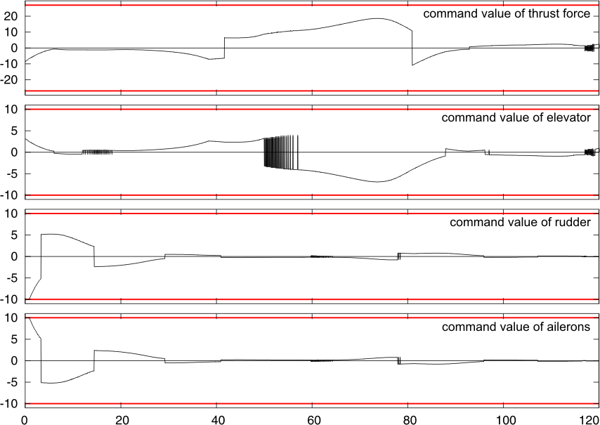
Below, the simulation results are given. In Fig.4, command levels of the controls are shown. Figure 5 contains the graphs of the positions of the control devices. The red lines denotes the maximal deviations of the control devices. One can see that these levels mostly are not reached. In the graphs, there are two period of intensive control: at the beginning of the process and in the middle. The starting activity is conditioned by eliminating initial deviations from the nominal glide path. The activity in the middle is connected to overcoming the microburst.
In Fig.6, the realizations of the wind disturbance are shown. Here, the red lines denote the critical level of the disturbance, under which there is guarantee of reaching the terminal set. It can be seen, that the real disturbance excesses this level.
Additional video (aircraft-simulation.avi, 3.63Mb) demonstrates the corresponding aircraft motion. At the top, there is a side view, the green line denotes the nominal glide path, the black one shows the ground and the runway. In the middle, one can see an upper view. At the bottom, at the left, the rear view is shown; the green point denotes the nominal position on the glide path. At the bottom, at the right, schematically, command signals (red lines) and current position (green lines) of the control devices are given.
|
| Fig.4. Command levels of controls |

|
| Fig.5. Values of controls |

|
| Fig.6. Realization of the wind disturbance |
References
1. Patsko V.S., Botkin N.D., Kein V.M., Turova V.L., Zarkh M.A. Control of an aircraft landing in windshear // Journal of Optimization Theory and Applications, Vol.83, No.2, 1994, pp.237-267.
2. Ganebny S.A., Kumkov S.S., Patsko V.S., Pyatko S.G. Robust Control in Game Problems with Linear Dynamics. Preprint. Institute of Mathematics and Mechanics, Ekaterinburg, Russia, 2005, 53 p.
3. Ivan M. A ring-vortex downburst model for real-time flight simulation of severe windshear // AIAA Flight Simulation Technologies Conf., July 22-24, 1985, St.Louis, Miss., pp. 57-61.