The talk is divided into three parts as follows.
First, we talk about the problem statement, namely, an M-approaching DG and the maximal stable set W.
Then we describe some known results on the problem: a corresponding Cauchy problem for Hamilton - Jacobi - Bellman - Isaacs equation, Hopf formula, and Pshenichnyi - Sagaidak formula. Here, we introduce an operator Tτ over the set M known as a "programmed absorption operator". This operator has a semigroup property for a convex set M.
Next, we present our results for the problem concerning the DG in the plane and nonconvex terminal set M. There are a theorem, a proposition and some examples that illustrate the theorem.
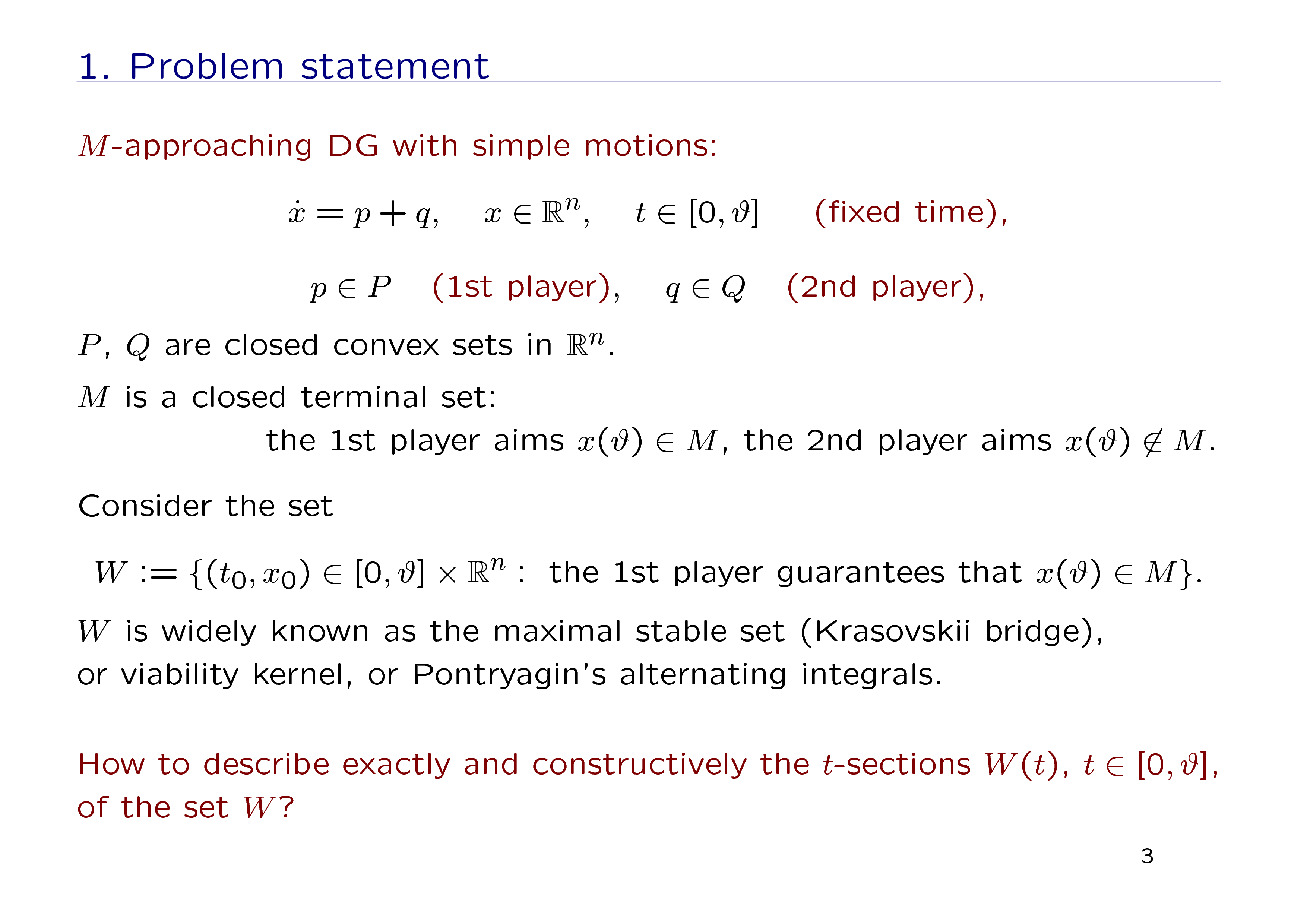
Here, we begin with the problem statement. Consider a differential game with simple motions and a fixed terminal time ϑ. Here, p and q are controls of the first and second player correspondingly; P and Q are closed convex constraints on the players' controls; M is a closed terminal set. The 1st player aims to bring the phase vector to the terminal set at the instant ϑ; the aim of the second player is opposite.
Consider the set W formed by initial positions whence the 1st player guarantees entering the state x(ϑ) into the set M. The set W is widely known in various formalizations of DGs and called the maximal stable set (Krasovskii bridge), or viability kernel, or Pontryagin's alternating integrals.
Our main question is: how to describe exactly and constructively the t-sections of the set W keeping in mind the case of nonconvex M ?
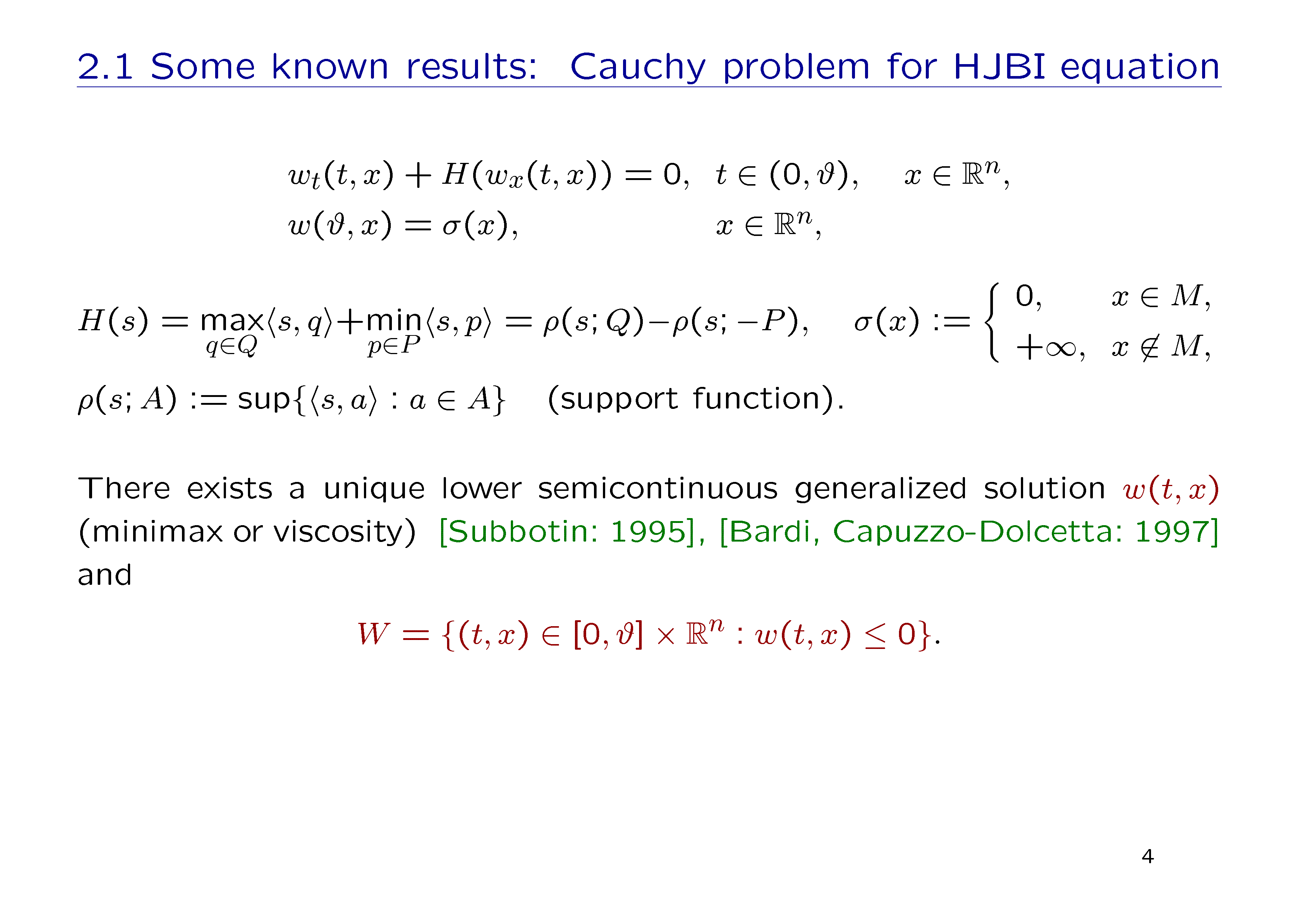
Here, we describe some known results on the problem.
The DG is connected with the HJBI equation and a boundary (terminal) condition. Here, the Hamiltonian is a difference between two convex support functions, and the terminal data function σ is the indicator function of the terminal compact set M.
So, we have a terminal Cauchy problem with nonconvex Lipschitzian Hamiltonian and lower semicontinuous terminal data. It is known that, in this problem, there exists a unique lower semicontinuous generalized solution w(t,x) (in the viscosity or minimax sense). Its connection with the maximal stable set W is shown on the slide.
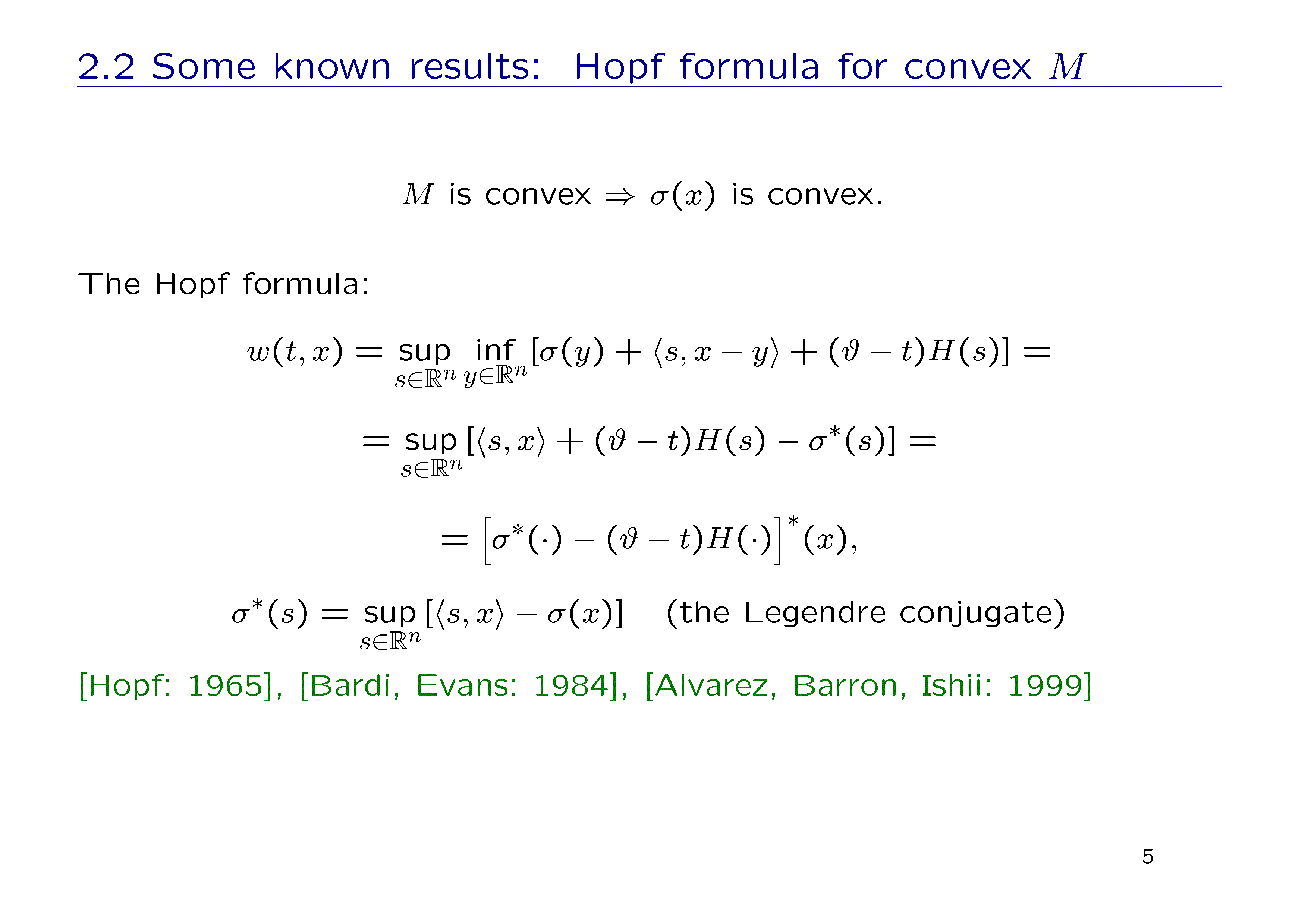
The widely known result concerned the convex data function σ (or the convex terminal set M, that is the same) is the Hopf formula. This formula represents the generalized solution w(t,x). There are three different ways to write the Hopf formula, and two of them use the Legendre conjugate transformation.
Here, there are some references for the Hopf formula concerned different kinds of generalized solutions.
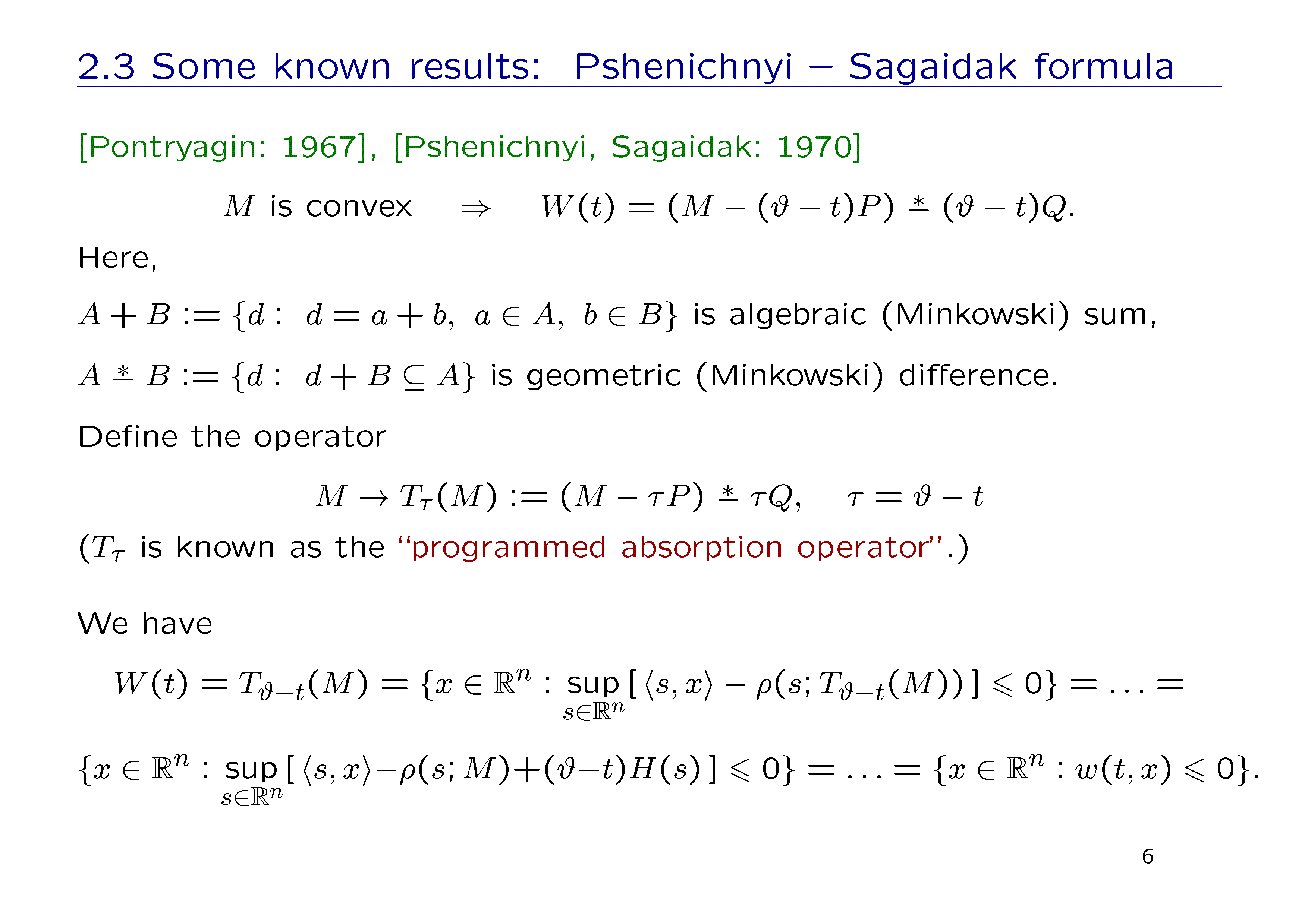
Let's turn to another well-known way to describe the set W developed in the works by Pontryagin and Pshenichnyi & Sagaidak. Now for simplicity, we begin with the convex case.
If M is convex, then we have a representation for a t-section of the set W. Here, we use the notations of algebraic sum and geometric difference.
We can rewrite the formula for W(t) defining the operator Tτ that is known in Russian literature as the "programmed absorption operator". Here, we use the notation τ for the backward time.
So, the above mentioned formula (note that the formula is written for the convex M) can be transform to the presentation via the generalized solution given by the Hopf formula.
Our new results consist of conditions that provide the representation formula for a nonconvex set.
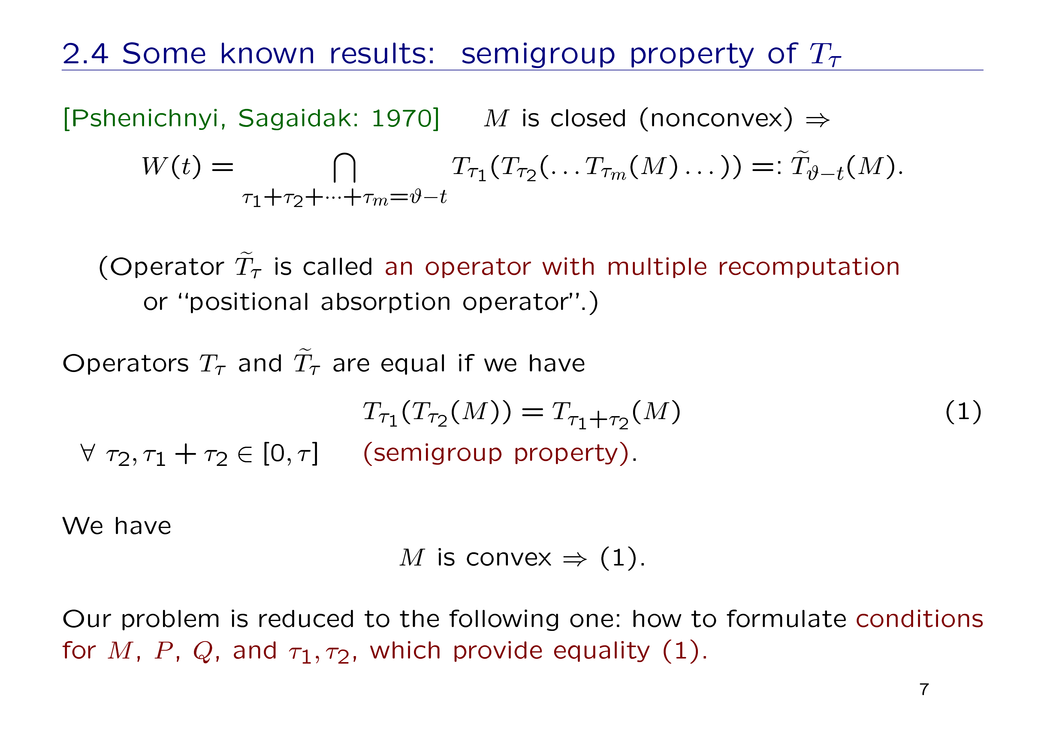
For the case of a nonconvex M, a more complex representation of the t-sections of the set W by the programmed absorption operator Tτ is known. Namely, we must use an operator with multiple recomputation by the operator Tτ and intersection of the results over all possible finite decompositions of the segment. Note that the operators Tτ and the operator with multiple recomputation are equal to each other if we have the property (1) called a semigroup property. For a convex M, this property is true.
So, our problem can be reduced to the following one: what kind of conditions for M, P, Q and τ can provide the equality (1).
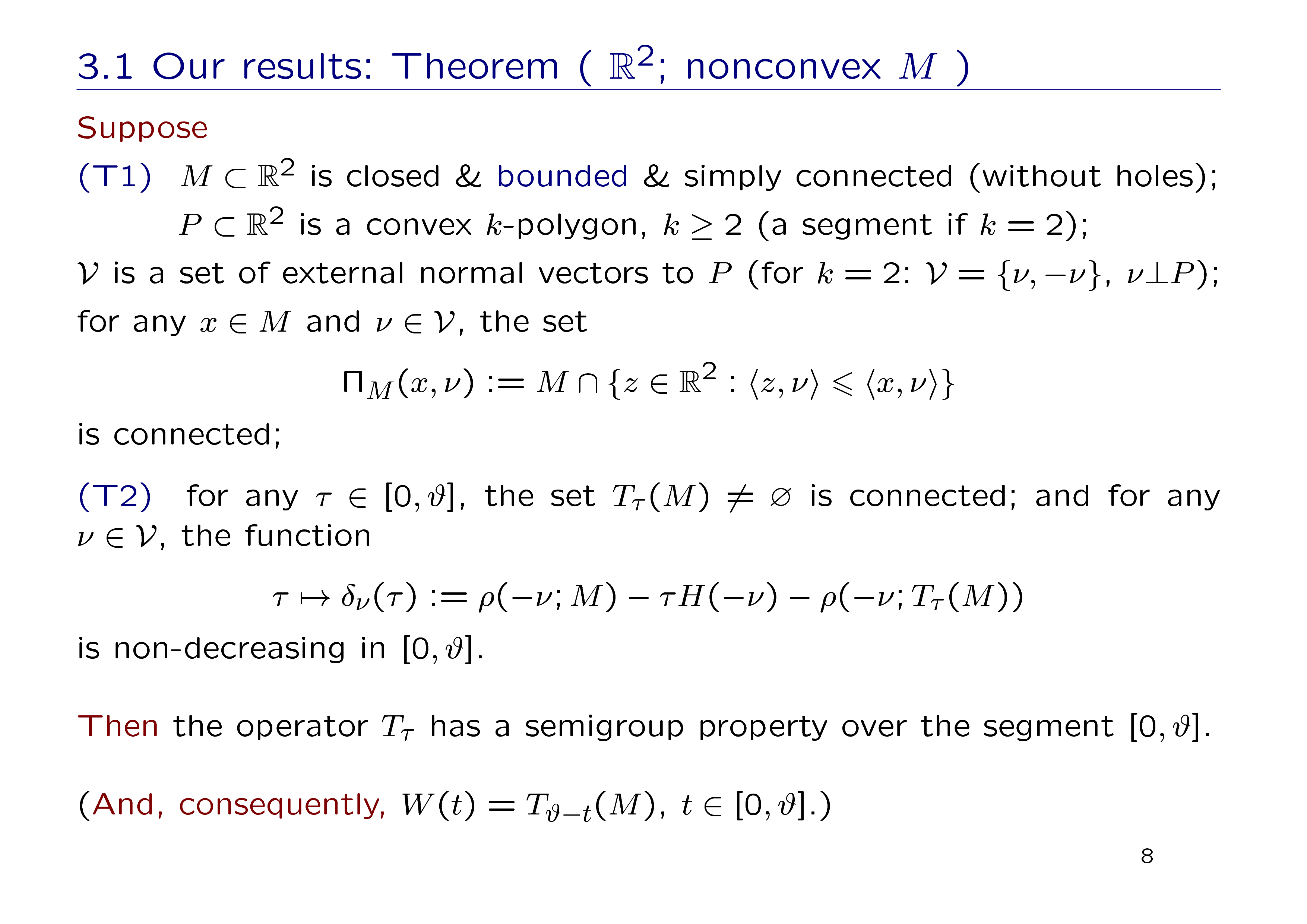
Let's formulate our main result on this problem. The theorem shown on the slide was proved for the DG in the plane.
Suppose two groups of conditions are fulfilled.
The first group (T1) consists of geometric conditions on the terminal compact set M and on the constraint P of the 1st player.
The second group (T2) of the conditions is connected with properties of operator Tτ on parameter τ. Here, the notation ρ means a support function.
Assuming these conditions, we claim that the operator Tτ has the semigroup property over the segment [0, ϑ]. And, consequently, we get an extension for nonconvex M of the representation formula mentioned above.
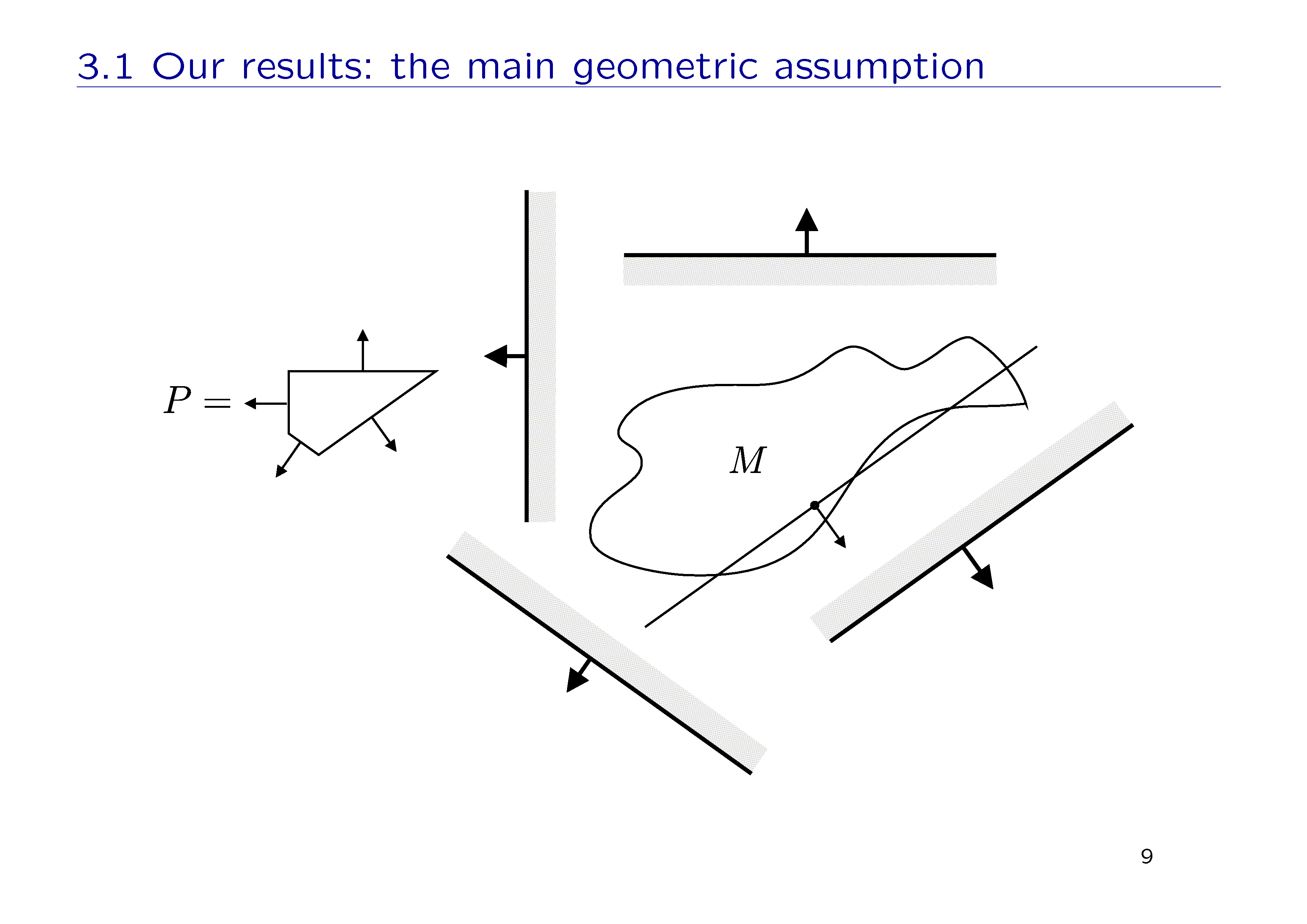
This picture illustrates the main geometric assumption of the theorem.
As an example, consider the constraint P of the first player and the terminal set M, which are shown on the slide. You can see that any intersection of M with the considered half-planes is connected.
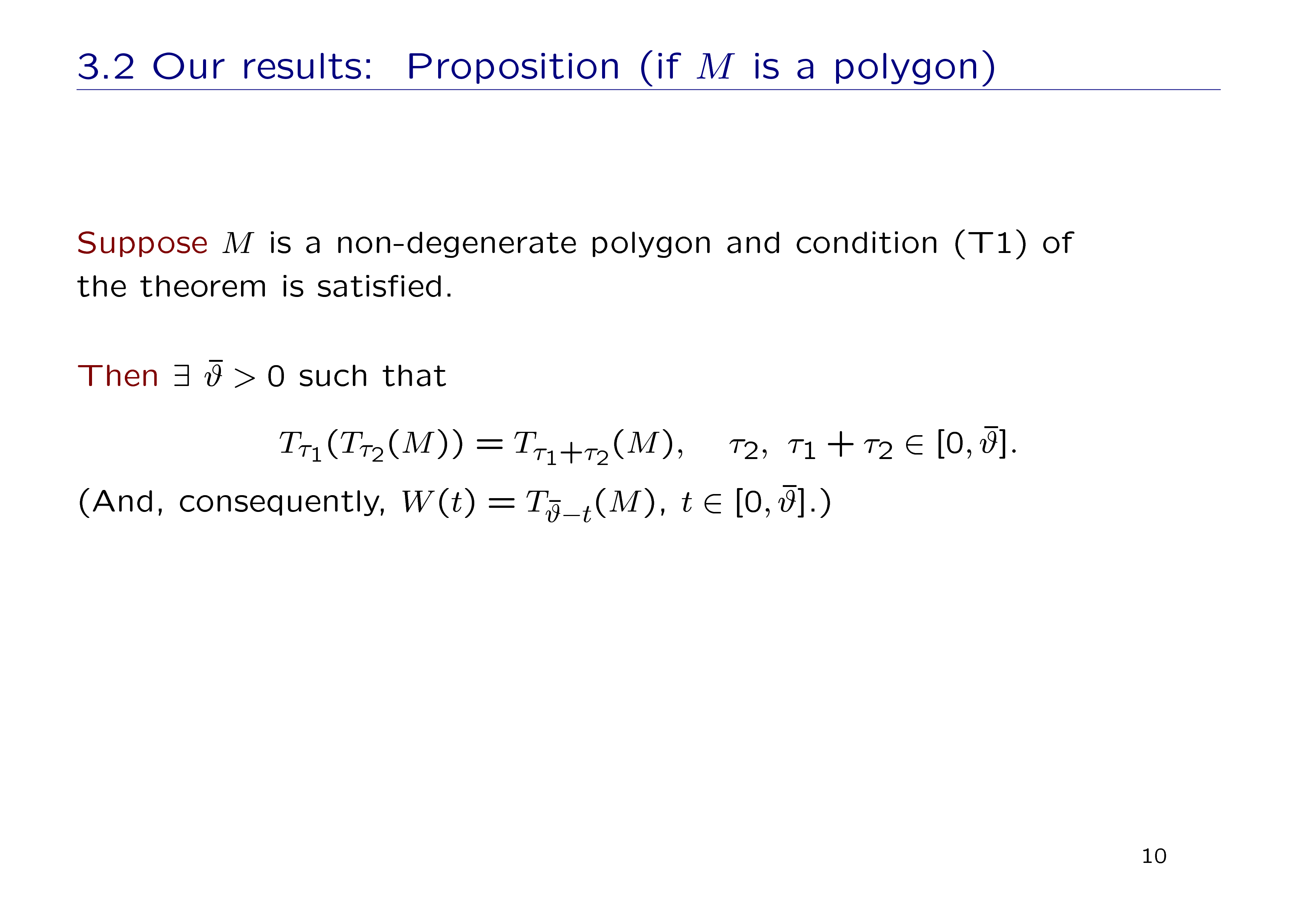
For the case when M is a non-degenerate polygon, the proposition on the slide is valid. In this case, we suppose that only the geometric conditions (T1) of the theorem are satisfied.
Then we claim that there exists such a time segment that the semigroup property of the operator Tτ over the segment is true. This means that the representation formula remains true over the segment.
Finally, we show some pictures that illustrate an importance of any condition of the theorem. If we eliminate any of the mentioned conditions, we can construct an example without the semigroup property.
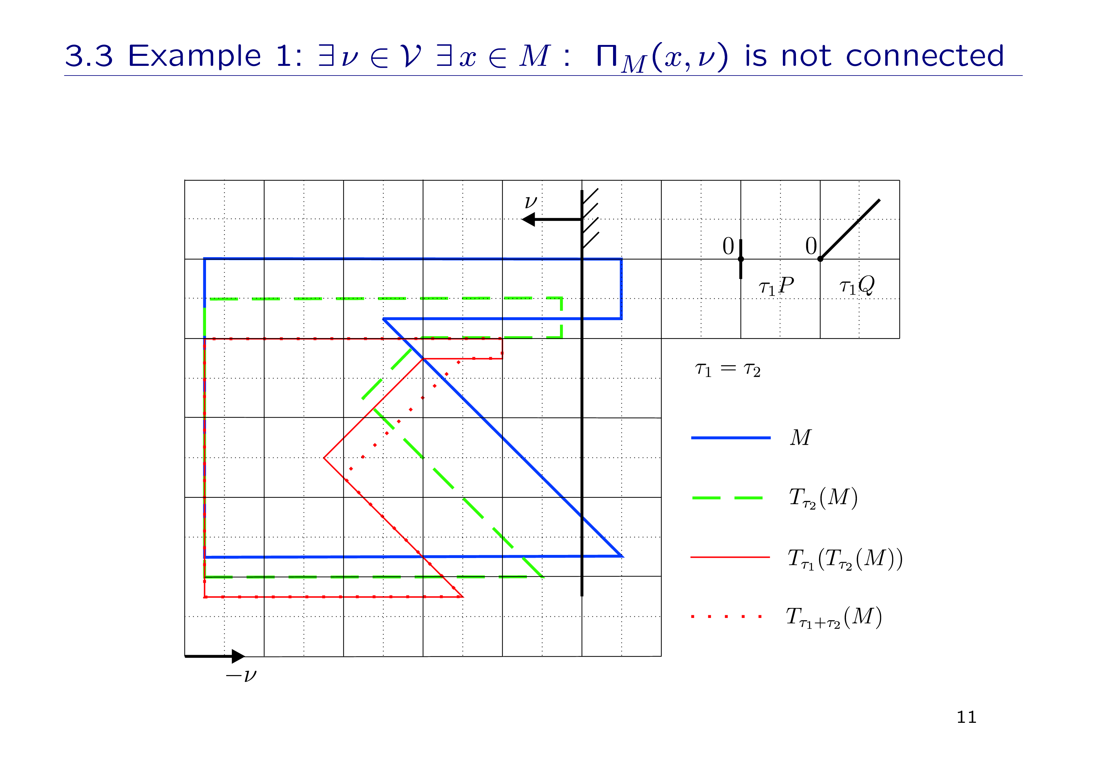
In the first example, we eliminate the main geometric assumption. Here, the set M is like a rectangle with a triangle excision at the right; P and Q are segments; and the set ΠM for a point x with a normal vector ν (normal to P) is not connected.
We make a geometric construction of image of M under the operator Tτ for the time parameters τ2 and τ1 sequentially (with the recomputation at the instant τ2, red thing line), and for the time parameter τ1 + τ2 (without a recomputation, painted by red dotted line). As we can see, the results are different.
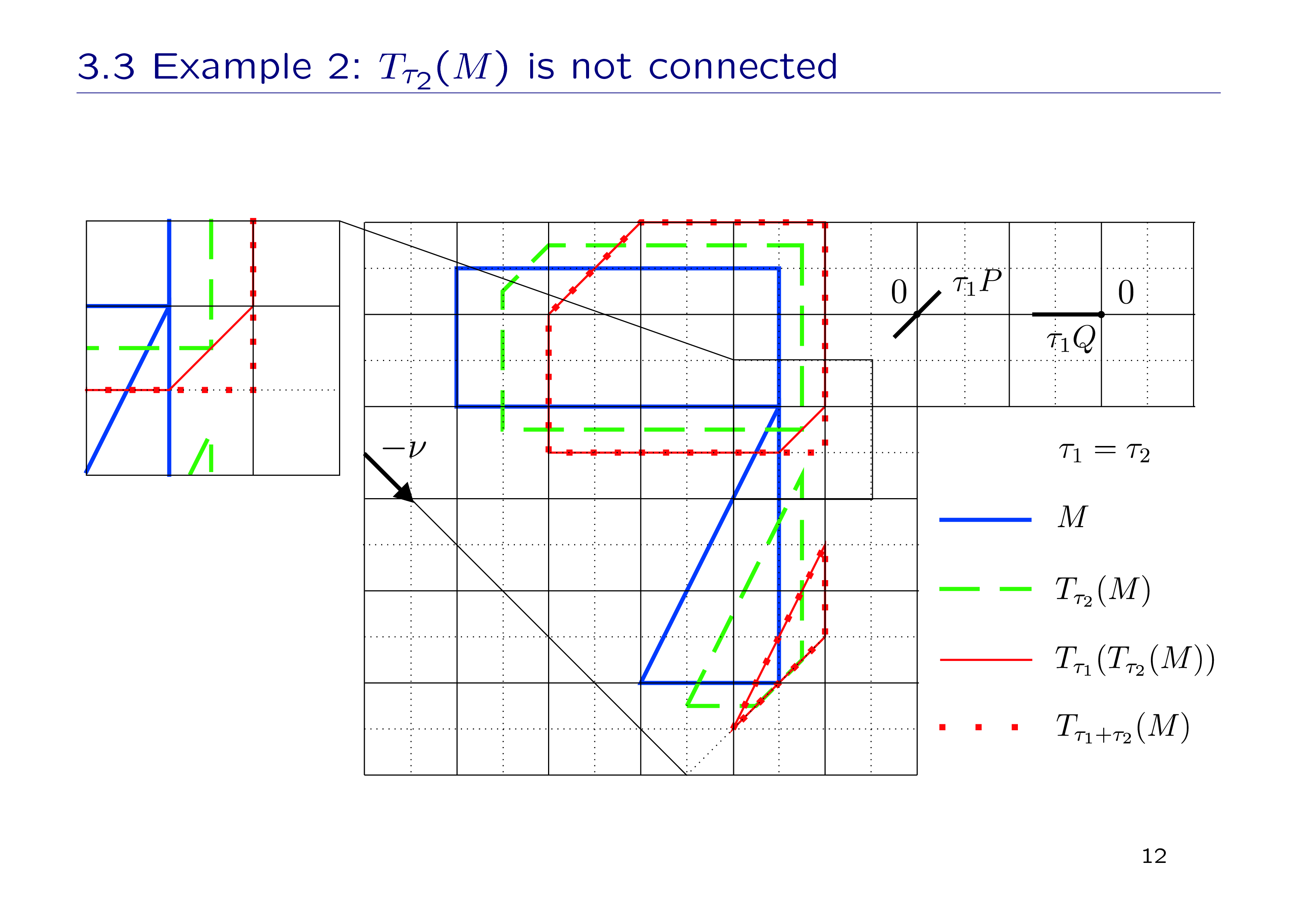
In the second example, we eliminate the assumption of connectedness of the intermediate set (green dash line). Here, the set M consists of two parts (a rectangle and a triangle), which intersect by one point and the intermediate set is not connected. The same geometric construction gives the images of M under the operator Tτ with the recomputation at the intermediate instant τ2 and without a recomputation. The images are different (and are not connected).
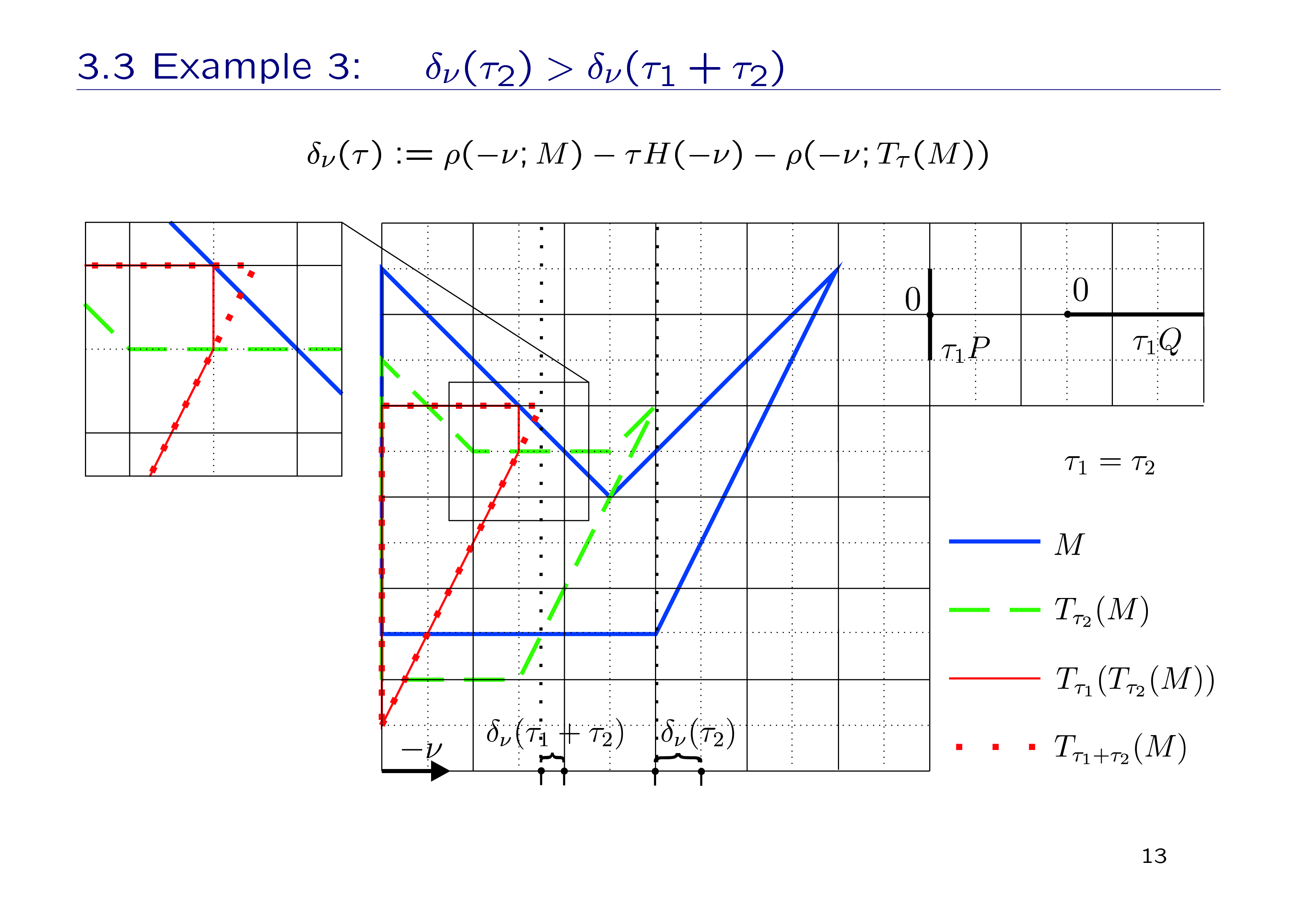
In the third example, the function δν from the second group of the assumptions is not non-decreasing. Here, the set M has a configuration with some kind of "a tooth" or "a peak". Here, the values of the function δν at the intermediate value τ2 and final value τ1 + τ2 are shown. And the images of M under the operator Tτ with the recomputation and without a recomputation are different.
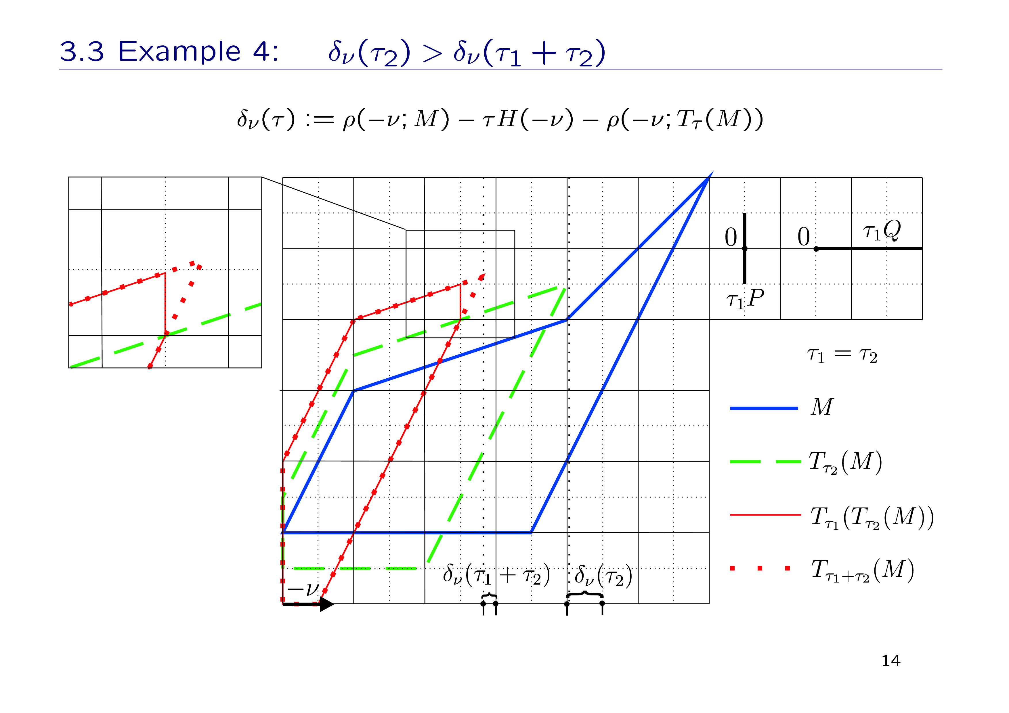
The fourth example is on the same topic as the previous one, but for other configuration of M. Here, "the tooth" (or "the peak") is not specified evidently.

Here, you can see the main references in our work.