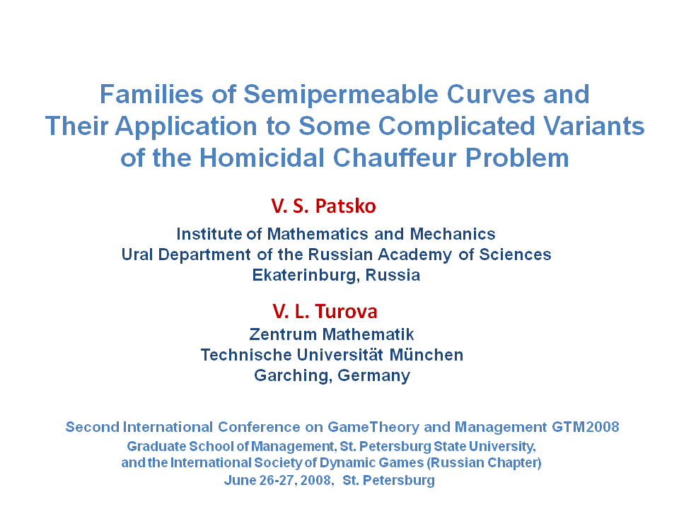
This is the simplest model of the car's dynamics. It is called Dubins' car. Here xp, yp are the coordinates of the geometrical state, θ is the angle of velocity vector to the vertical axis, and u is the control.
Fix the origin as the initial point. Let the vector of the initial velocity is directed upwards along the vertical axis. Then the time-limited reachable sets (or reachable sets by given time) look like it is shown in the figure. The fronts of these sets propagate by going around two dark arcs.
Let us imagine a real function whose value at every point is the propagation time required for the front to reach the point. We call such a function as the value function. It is clear that the value function determines the optimal time of reaching the origin, the direction of the velocity vector at the origin being specified. The value function is discontinuous on the above mentioned arcs.
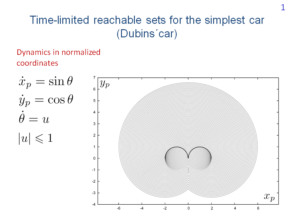
Consider Isaacs' homicidal chauffeur game. Dynamics of player P is written to the left, dynamics of player E is to the right. The velocity of player E is bounded by a number ν.
Put the origin of the reference coordinate system at the current position of player P. Then the current state of player E is described by the system of the second order. Player P strives to bring the phase vector to a given target set as soon as possible. Player E has the opposite goal. In the classical setting, the target set is a circle centred at the origin.

This slide shows level sets and graph of the value function for the homicidal chauffeur game. The value function is discontinuous on two dark lines.
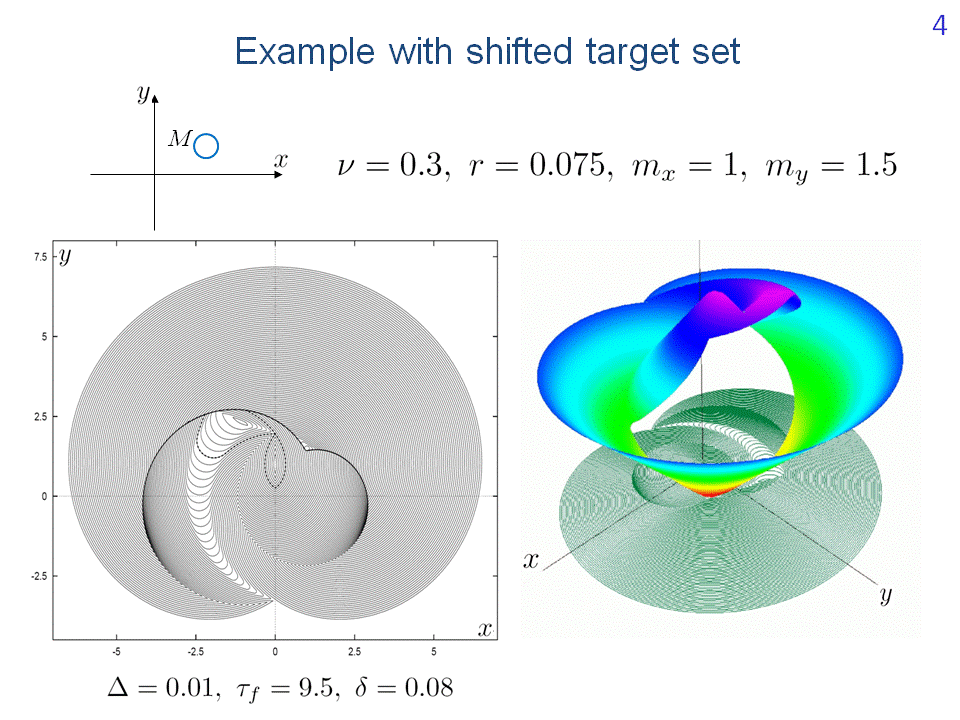
Let us shift the centre of the target set. Consider again the discontinuity lines of the value function. We have two lines as it was before. The following question arises. Would it be possible to predict discontinuity lines of the value function without solving corresponding time-optimal game?
The answer is "yes", and it is related to the investigation of families of smooth semipermeable curves in the plane. The smooth semipermeable curves are defined by the dynamic equations and constraints on the controls of the players only.
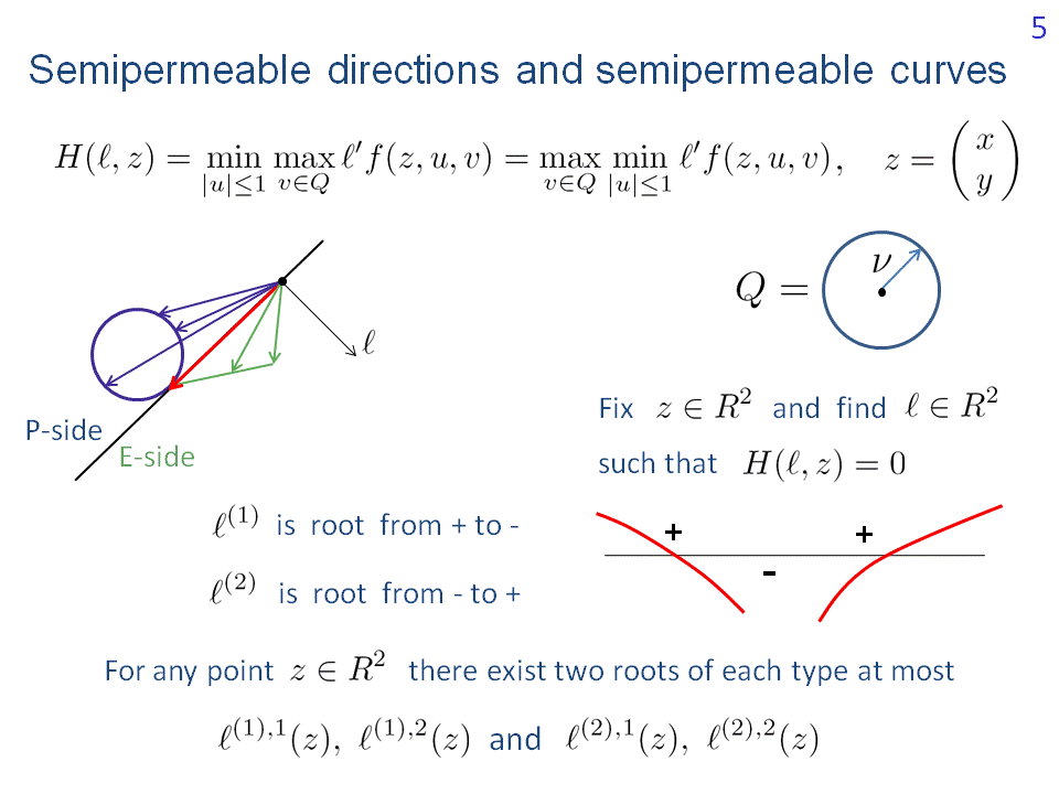
Consider minmax Hamiltonian function of the controlled system. Here, f is
the right hand side vector of our system. Symbol z stands for a point in the
plane x,y. The function
Choose a counterclockwise direction as a standard one for the boundary of the unit circle. For every point z find a unit vector l such that the Hamiltonian becomes zero. We consider the first type root from plus to minus and second type root from minus to plus. For the dynamics considered, it is proved that no more than two roots of each type can exist at every point.
Let
The existence of the root can be explained using the velocity vectograms of players P and E. Namely, a root exists, if and only if the vectograms are separated.
The unit vector of the system velocity corresponding to the extremal control for the first (second) type root is called the semipermeable direction of the first (second) type. The semipermeable direction of the first type is obtained by a clockwise rotation of the vector l through the anlgle π/2. For the second type semipermeable direction, a counterclockwise rotation takes place.
A smooth curve is called the first type semipermeable curve if the tangent vector at every point is the first type semipermeable direction. Similarly, the second type semipermeable curves are introduced.

Based on these facts, we can compute the semipermeable curves as solutions of the ordinary differential equation shown in the upper part of this slide. Here, Π is the operator which rotates the vector by the angle π/2. We use a clockwise rotation for the case j=1 (the first type root) and counterclockwise rotation for the case j=2 (the second type root).
On the left, regions with different types of roots are shown. The domains of the first type roots are depicted on the right.
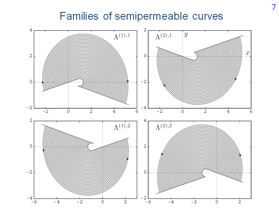
Here, four families

Let us go back to our two examples of level sets. For the left picture, the
target set is a circle centred at the origin. For the right picture, the centre
of the target set is shifted. Now, we can clearly see that the discontinuity
lines are semipermeable curves. The right arcs in both pictures are from family
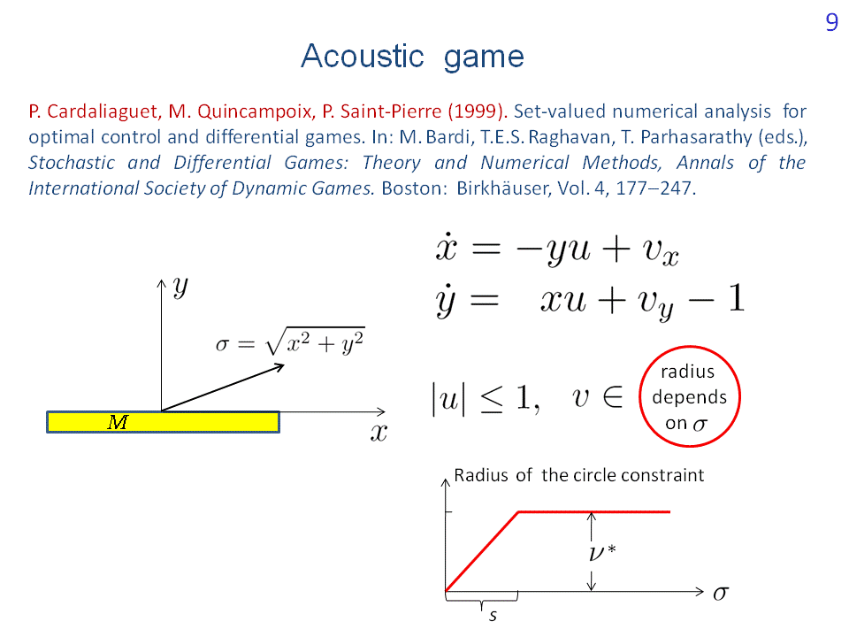
P. Cardaliaguet, M. Quincampoix, and P. Saint-Pierre have considered a variant of the dynamics in which the radius of the circle constraint of player E depends on the distance σ of the current state to the origin of the reference system. The applied aspect is the follwing: the object E should not be very loud if the distance between him and player P becomes small. The dependence of the constraint on the distance σ is shown in the right lower picture.
The differential game with such dynamics was called the acoustic homicidal chauffeur game. Different target sets were considered, also in the form of a rectangle stretched along the horizontal axis

Here, the level sets and the graph of the value function are shown for one particular case. The values of the game are infinite outside the region filled out with the level sets. We can precisely detect to which family of semipermeable curves belong those curves that form the boundary of this region and touch the target set. But what about the hole inside? Would it be possible to describe it effectively without the computation of level sets?
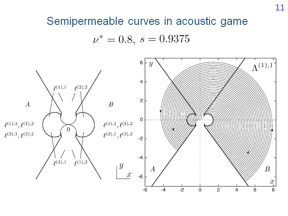
To describe the hole, one should study the families of semipermeable curves
of the acoustic game very thoroughly. Let us show, for example, the
semipermeable curves for the following parameters of the dynamics:
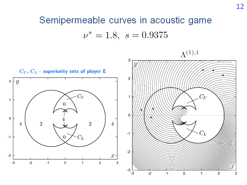
Let now reinforce player E by taking a larger value of parameter
ν*. In this
case, the family
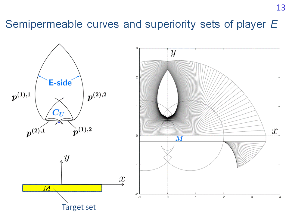
In this way, we can give a description of the hole. The picture to the left shows those semipermeable curves which form the boundary of the hole. It consists of two first type and two second type semipermeable curves. These curves can be constructed precisely. On the contrary, when constructing level sets, the time near the boundary of the hole goes to infinity. This makes the description of the obtained limit problematical.
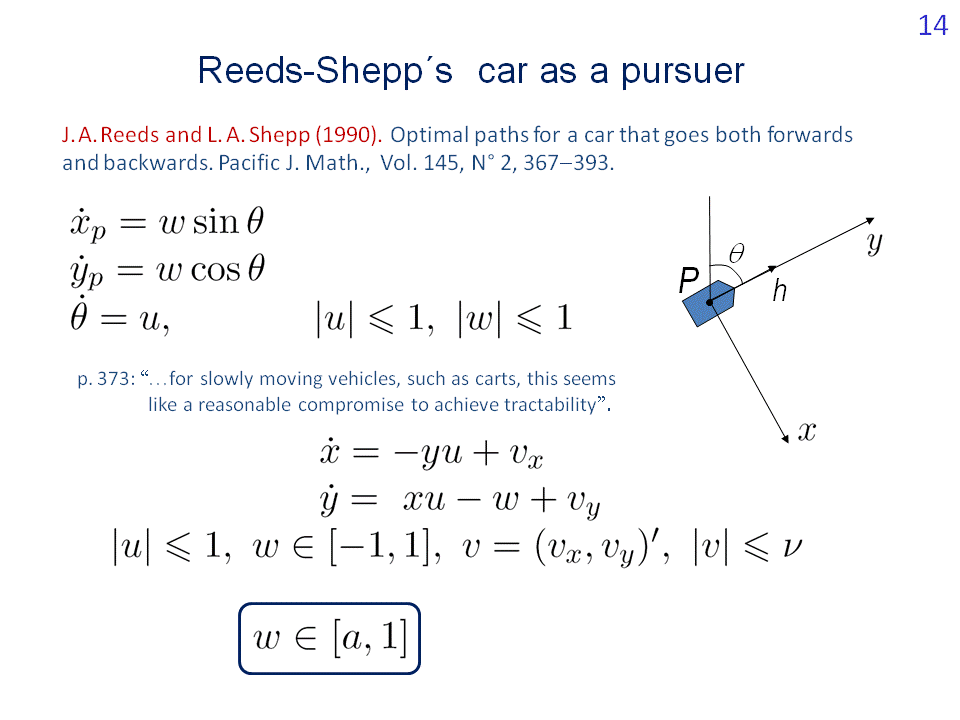
In the paper by J. A. Reeds and L. A. Shepp, a model time-optimal problem for a more agile car that can change his velocity vector instantaneously (by means of additional control w) was investigated. On the slide, a quote from this paper is given.
One can replace Dubins' car in the classical homicidal chauffeur game by
Reeds-Shepp's car. Moreover, we can consider an intermediate case using a
parameter a that specifies the lower bound on the linear velocity of player P.
If a=1, the classical homicidal chauffer game is obtained. For

For the classical variant of the homicidal chauffeur dynamics (which
corresponds to

For the more agile car, instead of two circumferences we deal with the arcs of four circumferences and with their involutes.
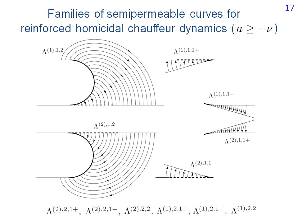
This slide corresponds to the case where a ≥ -ν. The first and second type families generated by the arcs of two right circumferences are shown. We obtain three first type families and three second type families. Six symmetrical to them families are generated by the arcs of two left circumferences. All together, twelve families exist.

In the case a ≤ -ν, the number of smooth semipermeable curves increases. Here, one can see the first type families generated as involutes by the arcs of two circumferences. In the case considered, sixteen families are obtained.
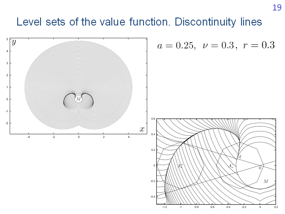
On this slide, results of the computation of level sets of the value function are presented for a = 0.25. On the right, an enlarge fragment of the computation is given. The left discontinuity line is a smooth junction of two semipermeable curves of the second type. Using the knowledge about the families, we can precisely determine where the left discontinuity line terminates. The right discontinuity line is symmetrical to the left one. It is composed of two semipermeable curves of the first type.

Here, the value of parameter a is less than -ν. Using the information about the families of semipermeable curves, we can predict before the computation of level sets that four short curves emanating from the points c, d, e, f are discontinuity lines. The upper curves should terminate at the horizontal line y=0.3, the lower curves finish at the line y=-0.3.
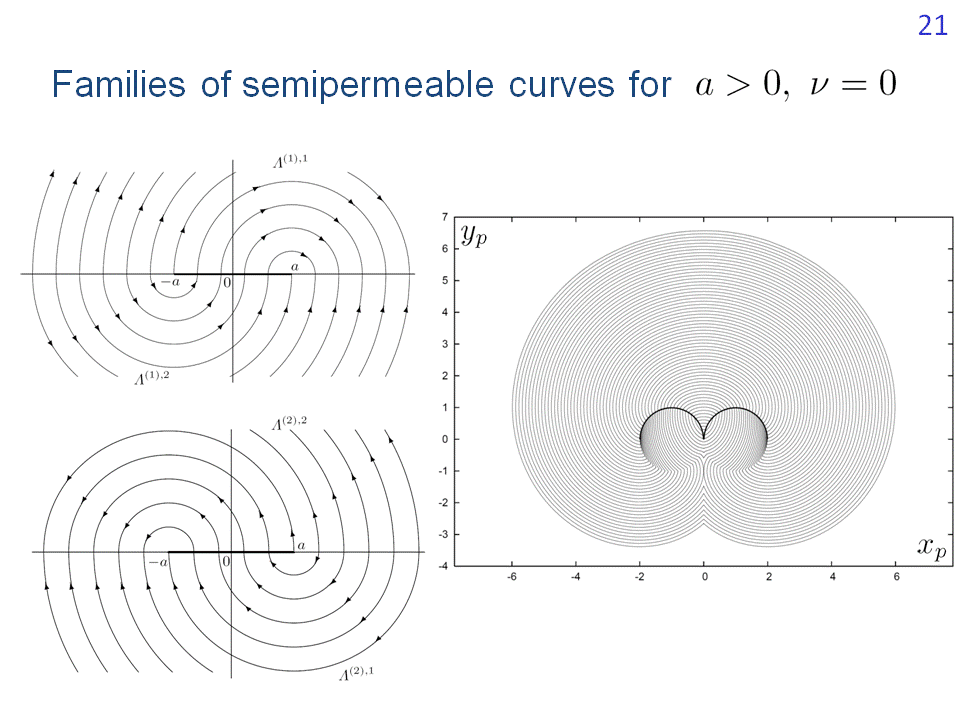
To complete, let us demonstrate the simplest case where player E is immovable and the value of the parameter a is positive. In this case, we have four families of semipermeable curves. Every semipermeable curve is a semicircumference.
Three related papers by the authors are presented.