Analytical and numerical
study of the dolichobrachistochrone problem
Title

This talk was presented at the conference
"Viscosity Solutions and Applications" &
"Analysis and Control of Deterministic and Stochastic
Evolution Equation", Bressanone-Brixen, Italy,
July 3-7, 2000.
The paper is devoted to the analytical and numerical
study of a time-optimal game problem in the plane. This problem
is a game extension of the model brachistochrone problem.
The classical brachistochrone problem
Slide 1
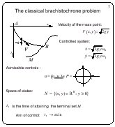
Let A and B be arbitrary points in the vertical plane. One looks
for a curve connecting A and B such that a mass point being
started from A with zero initial velocity attains B along this
curve for a minimal time. In general case, the terminal point B
is replaced by a given terminal set M. For any trajectory, the
velocity of the mass point at (x, y) is
(2gy)1/2, where g is
the gravitation constant.
The brachistochrone problem can be reformulated as a control
problem: instead of choice of the trajectory, we assume that the
magnitude of the velocity is (2gy)1/2 and the direction is
defined by the unit vector u. Thus, u is chosen from the unit
circle P. The problem is considered for y > = 0. The objective
of the control u is to minimize the time of attaining a terminal
set M. This control problem is equivalent to the brachistochrone
problem.
Isaacs' game statement of the problem
Slide 2
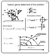
When considering the brachistochrone problem in the book
"Differential games", Isaacs introduced a disturbance
influencing the dynamics of the system. The disturbance can be
interpreted as a second player whose objective is to increase the
time of attaining the terminal set.
Isaacs considered the first quadrant as the state space. The
terminal set was the positive semiaxis y. So, it was unbounded.
The vectograms of the players were: the circle of radius
(2gy)1/2
for the first player and the diagonal of a square with the side
w for the second player. The first player minimizes the time of
attaining the terminal set M, the second player has the
opposite objective.
It is clear that the coefficient (2g)1/2 does not play any
role, hence it can be replaced by 1.
A solution to this differential game was given by Isaacs in his
book. However, this solution is not fully correct. Namely,
Isaacs supposed that the value function is infinite below the
horizontal line y = w2. Above this horizontal line,
the solution is defined by a switching line of the second player. On one side
of the switching line, the second player utilizes one of two
extremal controls. On the other side of the switching line, he
uses the other extremal control.
Improved solution to the Isaacs' problem
Slide 3
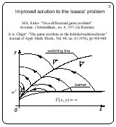
Lidov pointed out to an error in the Isaacs' solution. Later on,
Chigir has improved the solution of Isaacs. The horizontal line
y = w2 is not a barrier,
as it was erroneously claimed in the Isaacs' book.
Namely, there are points below this line for which
the game is solvable. The correct form of the barrier is shown on
the slide. The optimal trajectories are breaking on the switching
line of the second player. The value function is differentiable
in the whole solvability domain.
It is interesting to modify the game statement of the
brachistochrone problem so that the value function would become
non-differentiable. Besides we wanted to find out whether
singular equivocal lines can arise in the game brachistochrone
problem. According to the book of Isaacs, equivocal singular
lines are inherent to differential games only.
Our statement of the problem
Slide 4
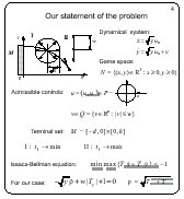
Let the vectograms of the players are of the following form: a
circle of radius y1/2 for the first player and a vertical
segment of the length 2w for the second player. The symbols
u1
and u2 denote control parameters of the first player in the
description of the system dynamics. The variable v is a scalar
control of the second player.
The terminal set M is chosen to be a rectangle of the height
h with the base edge on the x-axis. Since the right-hand side of
the dynamic equations does not depend on x, the location
of M
on the x-axis and its width do not play any essential role. This
implies that the solution has to be symmetric with respect to the
vertical line passing through the center of M.
A Bellman-Isaacs equation for this problem is written in the
lower part of the slide.
Thus, we will consider only the right half of the solution. We
begin with the case h > w2.
Fields of characteristics
Slide 5
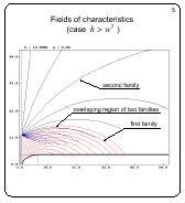
Using the Isaacs' method, we obtain three families of
characteristics that are constructed taking into account the
boundary condition on the terminal set. The characteristics of
the first, second, and third family emanate from the vertical
part of the boundary, from the right upper vertex of M, and
from the horizontal part of the boundary, respectively. The third
family consists of vertical lines. For all families, the
characteristics belonging to the same family do not intersect
each other. The first and second families overlap partially. The
second and third families adjoint each other smoothly.
Relations for the moving times along characteristics of all
families are obtained. Unfortunately, they do not define the
attainment time explicitly.
To obtain optimal trajectories, the characteristics of the first
and second families were processed additionally.
Solvability set and optimal trajectories
Slide 6
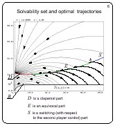
The singular dispersal line D was computed from the condition
that the attainment times along characteristics of the first and
second families are equal. Parts of characteristics computed
backwards are removed beyond intersection points with D. Each
point of D is a source for two optimal trajectories. The
construction of the dispersal line is stopped if it becomes
tangent to one of the trajectories of the first family. A point
corresponding to this situation is denoted by a on the slide.
The point a gives rise to a singular equivocal line E. The
property of equivocal line is that two optimal trajectories
emanate from every its point. One of these two optimal
trajectories goes into the upper region and arrives at the right
upper vertex of M along a characteristic of the second family.
The second optimal trajectory goes along the equivocal line up to
the point a.
The equivocal line is described by a first-order ordinary
differential equation.
The construction of the equivocal line is continued until it
meets a curve that bounds the second family from below. The
equivocal line approaches this curve tangentially. Let us denote
the common point by b. The point b divides the lower
bounding curve of the second family into two parts: the right
part is denoted by S on the slide. The curve S is a switching
line of the second player.
On the second stage of solving process, characteristics of the
Bellman-Isaacs equation are issued backwards from the parts
E and S of the singular line. At the moment,
complete description of these characteristics is absent (especially for the
characteristics issued from the equivocal curve E).
Thus, the first arc of the singular line that defines the optimal
solution possesses the dispersal property. This arc is computed
numerically. The endpoint a of the dispersal arc can not be
expressed analytically. The next arc of the singular line
possesses the equivocal property. It is a numerical solution to a
differential equation with a as the initial condition. The
endpoint of the equivocal arc is determined numerically too. The
third arc S is a switching line of the second player.
The value function is not differentiable on the arcs D and E,
and it is differentiable on the line S. The solvability region
of the problem is defined by the barrier line B that consists of
a curvilinear segment and a horisontal line whose y-coordinate is
equal to w2.
The barrier line is smooth. The value function is finite on the
curvilinear part of the barrier. The second player can prevent the
achievement of the terminal set whenever the trajectory starts
from any point that lies below the barrier line.
It was the description of the solution structure for
h > w2.
Now, we show how the solution changes if the value of the
parameter h decreases. The value of w is fixed.
Solution for h = 6.0, w = 2
Slide 7
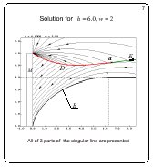
For this slide, h = 6. For the previous slide, h = 12.
Principally, the qualitative structure of the solution remains
the same. As before, the singular line consists of three arcs
and it is located over the barrier line B.
Solution for h = 4.4, w = 2
Slide 8
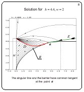
If h continues to decrease, the singular line approaches the
barrier line near and near. The limiting case where the singular
line touches the barrier is shown.
Solution for h = 4.3, w = 2
Slide 9
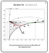
If h decreases further, the singular line breaks up: the
dispersal arc approaches the barrier B tangentially at the point
a1
but the equivocal arc emanates tangentially from another
point a2 lying on the barrier on the right from the point
a1.
Basically, the singular line consists of three parts as before.
Solution for h = 4.0, w = 2
Slide 10
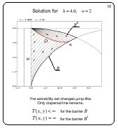
If h = w2, the solvability region changes jump-like.
An upper barrier line B* bounding the solvability region from above
appears. The equivocal arc and switching arc of the second player
disappear. It is interesting to observe that the value function
is infinite on the upper barrier line B*. The value function is
finite on the lower barrier B.
Solution for h = 3.5, w = 2
Slide 11
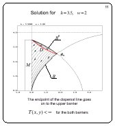
If h decreases, the solution structure remains the same: two
barriers define the solvability region. The endpoint of the
dispersal arc goes on from the lower barrier to the upper
barrier. The value function is finite for the both barriers.
These are results of our study based on the construction of the
singular line. The solution is not trivial. We have a code for
the computation of the singular line. The full exact proof for the
described solution structure is not completed yet. Nevertheless,
we are sure that our results are correct because they are in
agreement with the independent computation of level sets of the
value function. This independent computation utilizes an
algorithm based on the backward propagation of fronts.
Outlook of level sets of the value function
Slide 12
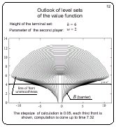
Here, level sets of the value function are presented for h = 6,
w = 2 . The curve consisting of the corner points of the fronts
is clearly seen. This curve coincides with our singular line. The
region that is filled out with the fronts coincides with the
solvability region. The accumulation of the fronts near the
horizontal line y = w2 means that the value function goes to
infinity when approaching y = w2 from above.
Enlarged fragment of the previous picture
Slide 13
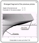
Here, a fragment of the previous picture is shown. More fronts
for the same time interval are presented.
Separation of the dispersal and equivocal
lines
Slide 14
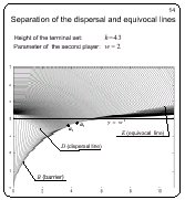
On this slide, a fragment of the collection of level sets of
the value function
is shown for h = 4.3. One can see that the curve composed of
corner points of the fronts is divided onto two parts. For
h considered, the division points a1
and a2 are close to earch
other.
Regions of accumulation of the fronts
Slide 15
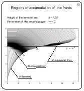
If h decreases, the point a1 and
a2 go away each from
other. An accumulation of the fronts arise over the terminal set
in the left part of the picture.
Appearance of the upper barrier
Slide 16
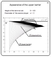
This picture is done for h = w2 = 4.
The accumulation of the
fronts in the upper part of the picture gives the upper barrier
B*. The solvability region changes jump-like.
Decrease of regions of the front accumulation
Slide 17
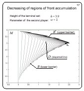
If h decreases more, the upper accumulation region of the fronts
reduces. The curve composed of the corner points of the fronts
meets the lower barrier as before.
Movement of the endpoint of the dispersal
line
Slide 18
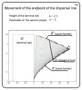
The computation is done for h = 2.5. The curve composed of
the corner points of the fronts meets the upper barrier.
Comments to the slides

L.V. Kamneva, V.S. Patsko
Institute of Mathematics & Mechanics
Ural Branch of RAS
S.Kovalevskaya str.16
620219 Ekaterinburg, Russia
e-mail:
kamneva@imm.uran.ru
patsko@imm.uran.ru
V.L.Turova
Center of Advanced European
Studies and Research
Friedensplatz 16
53111 Bonn, Germany
e-mail:
turova@caesar.de